BIO00087H Workshop 3: Genome assembly, gene finding and BLAST
Making a genome from raw reads
1 Learning objectives
The objectives of this workshop are:
- To gain skill and confidence with running software in Linux
- To learn concepts and terminology of genome assembly
- To learn about genome annotation pipelines
- To learn about BLAST (Basic Local Alignment Search Tool) and diamond
- Method 1:
jobs -l - Method 2:
top -u $USER
Try them both out some time today.
2 Introduction
2.1 From reads to chromosomes
NGS and 3rd generation sequencing machines produce reads, not joined-up chromosomes. If we want to know the complete genome sequence of a new species (all chromosomes, end to end), oursteps after sequencing will be:
- Check the quality of our read data
- Join the reads together to form contigs
- Join the contigs to form scaffolds (aiming for full chromosomes)
- Polish (correct) the contigs/scaffolds sequences
- Locate the protein-coding gene coordinates; starts, stops, exons and intron positions
- Locate non-coding RNA genes
- Annotate the genes (identify probable biochemical/cellular functions)
This genome can then be used for many different kinds of genome-scale analysis and other non-genomic research - like molecular cell biology. Today we will illustrate steps 1-7.
- Contigs: a contiguous sequence generated from determining the non-redundant path along an order set of component sequences. A contig should contain no gaps.
- Scaffolds: an ordered and oriented set of contigs. A scaffold will contain gaps.
- N50: The length of the shortest contig, in the set of contigs that contain 50% of the total assembly length. The image below will help to explain this.
- N90: As above but for 90% of the total assembly length.
- L50: The number of contigs that make up 50% of the genome.
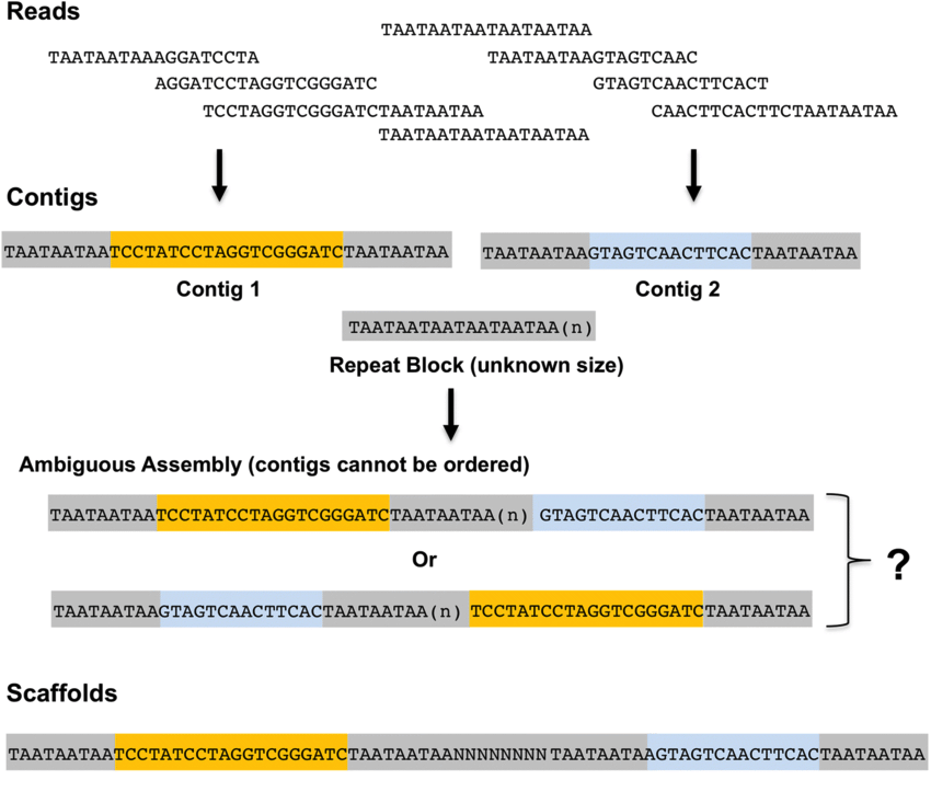
Figure 1. Assembly concepts explained Reads are the initial DNA sequences produced fom a sequencing machine. These may be short as shown here* (eg: Illumina technology), or long (eg:ONT/PacBIO). Reads are assembled into conigs. Contigs are ordered into scaffolds.
* Short reads are typically 150 nt long (not as short as shown here).
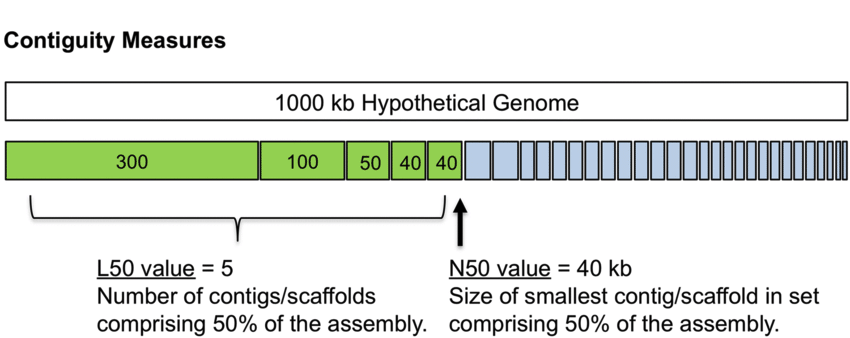
Figure 2. N50 The N50 is an assembly metric. In this example, the total assembly length is 100 kb, and the N50 is 8 kb. So 50% of our assembly is in contigs of the N50 value or larger. To calculate the N50, we order the contigs from the longest to the shortest. Then we add up their length, until the total length makes up at least 50% of our total assembly length. The L50 is the number of contigs that add up to 50% of the assembly length. Both N50 and L50 are simple, useful metrics.
3 Exercises
In this module it is OK to use AI to explain Linux commands and R code. Google Gemini is the University’s preferred generative AI, but Claude AI can be better and ChatGPT is also good.
But do not use an AI to
- write your report
- improve your report
- generate code for your report
If in doubt about what is OK ask us, or read the University Guidance on AI
3.1 Setting up
3.1.1 Directory set up
Start up the PC in Linux as last time, log in and open the Terminal window.
You should already have your own directory in
/shared/biology/bioldata1/bl-00087h/students/
If not, make one as described here.Change to your directory with:
cd /shared/biology/bioldata1/bl-00087h/students/$USER
Note: that $USER is a special variable that contains your username. It is easier to type your username in place of $USER.
Make a new directory for this workshop with:
mkdir workshop3Change to this directory with:
cd workshop3
3.1.2 File set up
Today we will use files from this directory:
/shared/biology/bioldata1/bl-00087h/data/L.braziliensis/genome/To place symbolic links for all files in this directory within your
workshop3directory, do this:
ln -sf /shared/biology/bioldata1/bl-00087h/data/L.braziliensis/genome/* .
- Don’t forget the dot
.at the end! - Check that everything worked by listing the files with
ls - You should now have symbolic links to these files (and some others):
- Lbraz-subset.fastq.gz
- Lbraz-subset.necat.config.txt
- Lbraz-subset.readlist.txt
Lbraz-subset.fastq.gz contains some Oxford Nanopore Technology (ONT) long read data from the protozoan parasite Leishmania braziliensis. The other files are required to run NECAT, a genome assembly software.
3.2 Assessing read data quality
It is important to assess the quality of your data before you use it. We will use the fastp tool for this. Fastp can also filter fastQ files to remove reads that you prefer not to use. You won’t need it today, but the fastp manual is here.
To run fastp:
- Load the module
module load fastp/0.23.4-GCC-13.2.0
- Run fastp
fastp --in1 Lbraz-subset.fastq.gz --out1 Lbraz-subset.filtered.fastq.gz --html Lbraz-subset.fastp.html --reads_to_process 1000 &> Lbraz-subset.fastp.output.txt &
- Note all the flags that we use:
--in1specifies the input file--out1specifies the output file name for the filtered reads--htmlspecifies the html format report file name
We capture the output using the &> symbols. This captures text output that would usually appear on the screen, and saves it to a file called Lbraz-subset.fastp.output.txt.
Here we use --reads_to_process 1000 to process only 1,000 reads, so the software runs quickly. If you run fastp for your project, omit this option to process all the reads.
To look at the fastp results, view the file Lbraz-subset.fastp.output.txt using:
less Lbraz-subset.fastp.output.txt
Note: When you have seen the file with less, press q to quit and return to the command line.
You will see various statistics about the reads:
- The total bases tells us how many nucleotides of sequence data are in this file.
- Since this is 1000 reads, what is the average read length?
- Q20 bases and Q30 bases described how many bases are above Phred scaled quality scores 20 and 30 respectively. Q20 means one error error per 100 nucleotides.
3.3 Genome assembly
Now we will assemble these ONT reads using the NECAT assembly software.
NECAT runs in three stages:
necat correctcorrects the raw readsnecat assemblegenerates contigsnecat bridgebridges (joins) contigs to create scaffolds and polishes (corrects base call errors) in the scaffolds.
3.3.1 NECAT files
NECAT requires two files to run.
- A config file. This contains details about what the software should do.
- A read list file. This contains a list of all the sequence reads to assemble.
You should have these files your working directory:
Lbraz-subset.necat.config.txt(contains all the settings to run NECAT)Lbraz-subset.readlist.txt(contains only a list of fastq sequence files to assemble)
Take a look at these files using less.
3.3.2 Running NECAT correct
- Load the NECAT module:
module load NECAT/0.0.1-GCCcore-12.3.0 - Run NECAT to correct the raw reads:
necat.pl correct Lbraz-subset.necat.config.txt &> Lbraz-subset.correct.log &This will take 5-10 minutes to complete. - Using
ls -Fwill show you what files you have, and mark directories with a forward slash (/) after the directory name. You should now have a directory calledLbraz-subset.assembly. All the assembly output file swill go here.
Wait for NECAT correct to complete before running the next step.
- Method 1:
jobs -l - Method 2:
top -u $USER
You might look at the contents of the file Lbraz-subset.assemble.log, or read ahead while you wait. Or talk to us about genomics!
3.3.3 Running NECAT assemble and brige
Once NECAT correct is complete, run NECAT assemble:
necat.pl assemble Lbraz-subset.necat.config.txt &> Lbraz-subset.assemble.log &When assemble is complete, run NECAT bridge:
necat.pl bridge Lbraz-subset.necat.config.txt &> Lbraz-subset.bridge.log &
Your assembly is complete. Well done. You now have some long ONT reads, assembled into contigs, and then into scaffolds.
The final set of contigs is in the file: Lbraz-subset.assembly/6-bridge_contigs/polished_contigs.fasta
It is within Lbraz-subset.assembly because this directory was defined in the config file Lbraz-subset.necat.config.txt as the output directory for the assembly.
3.3.4 Assembly quality assessment
There are many ways to assess the quality an assembly. A simple way is to look at the metrics that NECAT itself provides. These are at the end the log files such as Lbraz-subset.bridge.log. To view the last 11 lines of this file do:
tail -n 11 Lbraz-subset.bridge.log
You will see information something like this (but not exactly), telling us the number of contigs (counts), their total, maximum and minimum length, and the N and L values for 25%, 50% and 75% of the assembly lengths.
Count: 2
Total: 133018
Max: 124310
Min: 8708
N25: 124310
L25: 1
N50: 124310
L50: 1
N75: 124310
L75: 1
You can also check how many contigs your assembly has by looking at the final output file in your directory Lbraz-subset.assembly/6-bridge_contigs/polished_contigs.fasta. Use either less or grep -c '>' to have quick look.
3.3.5 This is a terrible assemby.
This assembly has just one or perhaps two contigs (resultsvary between runs). That can’t be right, because other Leishmania species have 35 or 36 chromosomes, so the enture genome can’t be contained in one length of DNA sequence.
This is because we used very few reads. To save time in the assembly process, we provided only 10% of the reads we had available for this species.
See Appendix 1 if you want to make an assembly of all the reads for your report.
3.4 Genome annotation
Once we have an assembled genome, the next step is to annotate the genome, to locate the genes and other features within the genome. Protein-coding and non-coding (eg: tRNA) gene-finding is a complex process, which utilities a variety of information, including:
- gene start and stop codons
- transcript data from processed mRNAs (cDNAs)
- homology between predicted proteins in the new genome and related genomes
- signals of non-coding RNA secondary structures
3.4.1 Annotation with AUGUSTUS
There are many tools to identify protein coding and non-coding genes. Today, we will use AUGUSTUS, which is simple and runs rapidly.
We will not get much from annotating the L. braziliensis assembly because it is such a terrible assembly. Instead, let’s annotate another Leishmania species assembly, Leishmania lainsoni.
A link the the assembly file Llainsoni_NMT.fasta would already be in your workshop3 directory. Check this with ls *fasta.
3.4.1.1 Running AUGUSTUS
To run AUGUSTUS, load the module:
module load AUGUSTUS/3.5.0-foss-2023b
Then run:
augustus --sample=10 --species=leishmania_tarentolae Llainsoni_NMT.fasta > Llainsoni_NMT.fasta.gff &
This will take about 2-5 minutes to run. Note that we use --species=leishmania_tarentolae. This is because a pre-constructed database for this species is available, but there is not one for Leishmania lainsoni.
Warning: Number of sample iterations ‘sample’=10 is low. Posterior probabilities will be only rough estimates.
You can check is augustus is still running with jobs -l. If you see a line with augustus in it, it is still running. If you don’t see this line, it has finished.
Once augustus is done, the output file is in the gff (general feature format) file Llainsoni_NMT.fasta.gff. Have a quick look at it using less. You will see it contains a lot of information about th e predicted genes and the proteins they encode.
You can extract the just the protein sequences from the gff output file, with:
getAnnoFasta.pl Llainsoni_NMT.fasta.gff
This will complete almost immediately, and produce the file Llainsoni_NMT.fasta.aa. Use less to have a quick look at this file.
To count how many proteins have been predicted in this genome do
grep -c '>' Llainsoni_NMT.fasta.aa.
grep command
The grep command searches for patterns in files. Here we use it to count (-c) how many lines in the file Llainsoni_NMT.fasta.aa start with the character > (which is how sequences are marked in FASTA format files). Each sequence has a header line starting with >, so this counts how many sequences (proteins) are in the file.
3.5 BLAST
BLAST (the Basic Local Alignment Search Tool) is one of the most used tools in bioinformatics.
BLAST finds regions of similarity between DNA or protein sequences. Each search we perform compares a nucleotide or protein sequence query to a sequence database (which can be DNa or protein). BLAST calculates how matches we should expect, and reports this as the E-value (the ‘expect value’).
Gene function prediction. Once we have found new proteins in our genome, we want to know what their biochemical functions are. By identifying similar proteins, whose functions we know from experimental data, we can infer that our ‘query’ protein has similar function to the ‘hit’ protein.
Identifying homologous genes for evolutionary analysis. Evolutionary biologists use phylogenetic trees to understand many processes. BLAST helps to locate proteins to build these trees.
To run a BLAST search you need:
- a query: a protein or nucleotide sequence that you want to find something similar to
- a database of protein or nucleotide sequences. This is where we look for the similar proteins/nucleotide sequences. This is just a list of protein/nucleotide sequences re-formatted for BLAST.
Proteins in the database that match the query are usually called hits.
3.6 Diamond: faster than BLAST
BLAST is good (and very flexible), but today we will use diamond, which is more than 100 times faster than BLAST for protein-protein searches.
We will use diamond to find which proteins in Leishmania lainsoni are very similar to proteins in budding yeast Saccharomyces cerevisiae.
http://sgd-archive.yeastgenome.org/sequence/S288C_reference/orf_protein/orf_trans_all.fasta.gz
3.6.1 Running diamond
We will now search every Leishmania lainsoni protein against every Saccharomyces cerevisiae protein to find potential orthologs (proteins that are similar by evolutionary descent). Here is how:
- Make symbolic links to all the yeast files in your working directory:
ln -sf /shared/biology/bioldata1/bl-00087h/data/yeast/* .
You should now have links to the files Scer.fasta.aa (S. cerevisiae proteins) and a pre-built diamond database of these yeast proteins (Scer.fasta.aa.dmnd) in your workshop3 directory.
Check you have these links with
ls S*Load the diamond module:
module load DIAMOND/2.1.9-GCC-13.2.0
- Run the search. Here we use
--id 70to specify that we want to see only hits that are ≥ 70% identical. If you omit this flag, diamond locates all protein matches.
diamond blastp --query Llainsoni_NMT.fasta.aa --db Scer.fasta.aa.dmnd --out Llainsoni-v-yeast.ident70.tsv --id 70
This will run very fast. The output file will be: Llainsoni-v-yeast.ident70.tsv
3.6.2 Evaluating diamond results
First, look at your output file with:
less Llainsoni-v-yeast.ident70.tsv
(press q to quit the less viewer).
And count how many hits we got with:
wc -l Llainsoni-v-yeast.ident70.tsv
Use grep -c '>' *.fasta.aa to find out:
- How many L. lainsoni proteins we used as queries?
- How many yeast proteins we searched against?
Why did we get so few hits?
The information in the Llainsoni-v-yeast.ident70.tsv output file of diamond is described in Table 1.
Table 1. Diamond standard output format. The bit score (bitscore) gives an indication of how good the alignment is; the higher the score, the better the alignment. The **expect value* (E-value) is a probability for how many alignments of this quality you would expect in a database of this size. The lower the E-value, the better the hit. E-values are similar to, but not the same as, p-values. Because outputs are simple tab-delimited files, it is easy to read these into R and analyse them.
| column | field | meaning |
|---|---|---|
| 1 | qseqid | query or source (gene) sequence id |
| 2 | sseqid | subject or target (reference genome) sequence id |
| 3 | pident | percentage of identical positions (in the alignment) |
| 4 | length | alignment length (sequence overlap) |
| 5 | mismatch | number of mismatches (in alignment) |
| 6 | gapopen | number of gap openings (in alignment) |
| 7 | qstart | start of alignment in query |
| 8 | qend | end of alignment in query |
| 9 | sstart | start of alignment in subject |
| 10 | send | end of alignment in subject |
| 11 | evalue | the ‘expect value’ (see below) |
| 12 | bitscore | the ‘bit score’ (see below) |
There are many things you can do with BLAST or diamond searches. See the After the workshop section for one example.
4 End
That is all for today. Today we learned:
- About genome assemblies
- How to run NECAT, a genome assembly tool
- How to run AUGUSTUS a genome annotation tool
- About using BLAST and diamond to search for proteins in one species (Leishmania) that are similar to another species (Saccharomyces)
- We can also use diamond to search larger data sets, such as all the proteins ever discovered
The power of such BLAST/diamond searches is that most proteins in Saccharomyces have been experimentally characterised. So, if we find a Leishmania protein that has a similar protein sequence to an experimentally characterised Saccharomyces protein, we have an excellent prediction for the Leishmania protein’s function.
5 After the workshop
5.1 Evaluating diamond results
Can you guess what kinds of proteins have not changed much since the > hundred million years since Leishmania and yeast diverged?
Let’s find out what kinds of proteins have not changed much since Leishmania and yeast diverged.
First extract the yeast gene names from your diamond output with:
cat Llainsoni-v-yeast.ident70.tsv | cut -f 2
Then go to the yeast genome database gene list query page.
Copy and paste the yeast genes from the diamond output into the box, and click CONTINUE.
That’s it!.
6 Planning for your report
The assessment for this module is a 2000 word written report. The bioinformatic data analysis section involves replicating and extending one of the data analysis workshops we teach during the module. The workshops are:
- Workshop 3: Genome assembly, gene finding and BLAST
- Workshop 4: RNAseq analysis
- Workshop 5: Single cell RNAseq
- Workshop 6: Population genomics
The guide to writing your report is here.
7 Appendix: Assembly, annotation and/or BLAST for your project
The manual for NECAT is here, and the original article is Chen 2021. You don’t need to read these for your report, but the manual might help if you are stuck.
7.1 Appendix 1. Making an assembly with all the ONT reads
To save time for this workshop, we only provided 10% of the reads we had for L. braziliensis. If you want to run genome assembly and annotation for your report, the full set of reads are available here:
/shared/biology/bioldata1/bl-00087h/data/L.braziliensis/genome
This directory contain these files, that you should copy into (or make symbolic links) to your report directory.
Lbraz-allreads.necat.config.txt
Lbraz-allreads.readlist.txt
Lbraz-minion.fastq.gz
Lbraz-promethion.fastq.gz
7.1.1 How to edit config files, filter reads and run an assembly
We now provide an example of the commands to run fastp, filter reads, calculate read coverage, run and assembly, and annotate that assembly here: make-gald-assembly-2024-12-07.txt. This is for a G. sulphuraria (red alga) assembly, but the commands will be the same for L. braziliensis, apart from the file names.
You can also find this file here /shared/biology/bioldata1/bl-00087h/data/G.sulphuraria/make-gald-assembly-2024-12-07.txt
We also provide a filtered We also provide a much smaller set of reads that have been filtered to keep only reads that are at least 10,000 nt long, and have a mean base quality score ≥ 20. These are ere:
/shared/biology/bioldata1/bl-00087h/data/G.sulphuraria/genome/ont-reads/gald.filt.len10k.avQ20.fastq.gz
‘Read coverage’ is how many times we have sequenced the genome. For example, if each region of the genome is sequenced by 10 reads we have ten times (10x) coverage. We usually need ≥ 40 x coverage for a reasonable assembly, and increasing this to ~100 x can improve it. After 100x, we often don’t see much gain.
7.2 Appendix 2. Assessing assembly quality with QUAST
Here’s what the experts do:
- Check the module is loaded with
module list - Use
-h(or--help). For example, typingquast -hwill show you the help page for QUAST. - Read the manual: Googling
quast manualwill usually find the manual. - Most command line software we use on Linux has a
--helpor-hflag.
For project work, we advise you to use QUAST (Quality Assessment Tool) to assess the quality of your assembly. Here’s how to do it:
- Load the module:
module load QUAST/5.2.0-foss-2022a(or usemodule spider quastif this doesn’t work) - Run QUAST:
quast --output-dir quast-results <assemby_contigs.fasta>
Here <assemby_contigs.fasta> is the name of your assembly file. For example, if you are using the L. braziliensis assembly, this would be quast --output-dir quast-results Lbraz-subset.assembly/6-bridge_contigs/polished_contigs.fasta.
- The directory
quast-resultscontains the results of QUAST. We find that thequast-results/report.tsvfile is the simplest to read.
7.3 Appendix 3. Annotating your assembly with AUGUSTUS
Load the AUGUSTUS module and run on your final assembly as above.
7.3.1 How accurate are the predictions?
AUGUSTUS reports the posterior probabilities of its predictions for genes. This is the likelihood that the prediction is correct, given the data.
The posterior probabilities are estimated using a sampling algorithm. The parameter –sample==n adjusts the number of sampling iterations.You may choose to improve the accuracy of the likelihood estimates by increasing the sampling, like so:
augustus --sample=100 --species=leishmania_tarentolae my.fasta > my.fasta.sample100.gff
More information about AUGUSTUS is here.
You can extract the probabilities of the CDS (coding sequences) from the gff format output file like so:
cat my.gff | grep -v '#' | grep CDS > my.CDS.gff
And the GFF file could be loaded into RStudio for analysis. The posterior probabilities are in the 6th column of this file. Plotting and comparing posterior probabilities between assemblies or different samplings could make for an interesting project.
7.4 Appendix 4. BLAST/Diamond work
When you have predicted protein sequences from your assembly, running diamond will give you some information about how the protein sequences from the L. braziliensis genome compare to another species.
You can obtain FASTA format protein data sets for 66 different Trypanosomatid species here:
/shared/biology/bioldata1/bl-00087h/data/L.braziliensis/leishmania-protein-data/trypanomatid_protein_sets
Identifying the most and least conserved proteins between L. braziliensis and one selected other species would be sufficient for the BLAST-searching component of a report.