#clear all the previous data
rm(list = ls())

#set working directory
#your working directory will be different!
setwd("/Users/dj757/gd/modules/BIO56I/workshops/gwas")

#load the data
load(url("http://www-users.york.ac.uk/~dj757/BIO00056I/data/gwas-data.Rda"))BIO00056I GWAS Workshop
This document now contains answers to questions.
1 Learning objectives
- Understand the principles of quantitative genetics.
- Appreciate how this alters our perspective on evolution.
- Learn how to design experiments that explore quantitative trait variation.
2 Introduction
2.1 Background
In the lectures, we learnt about quantitative traits and how to analyse them. To recap, quantitative traits are often described as complex traits because they are affected by genetic variation in many genes. The genetic variants in those genes each account for a small proportion of the trait variation. We usually assume that they contribute in an additive way (rather than more complex ways).
One good way to identify loci controlling quantitative traits is to perform a genome-wide association study (GWAS). GWAS experiments use diversity panels of individuals to identify genetic markers that are significantly associated with a trait of interest.
Using a diversity panel instead of a biparental mapping population ensures that linkage disequilibrium is low (segments of co-inherited DNA are small), and therefore resolution is high (QTL sizes are small), which helps to narrow down the regions containing the genes controlling the trait. Diversity panels also capture much more genetic variation.
Quantitative traits and evolution
Most traits are quantitative, and are caused by multiple genetic variants. This means that:
- We expect traits to adapt gradually, as a few variants change
- We do not expect to observe many strong selective sweeps
Glossary
Technical definitions for this workshop.
- Schizosaccharomyces pombe: Fission yeast; a haploid, unicellular fungus widely used as a model organism.
- GWAS: Genome-wide association study; a statistical approach to associate genetic variants with traits across a genome.
- trait: A measurable characteristic (phenotype), such as growth rate at high temperature.
- Manhattan plot: A plot of genomic position (x) versus −log10(P-value) (y) showing association signals across the genome.
- QTL: Quantitative trait locus; a genomic region containing variants that influence a quantitative trait.
- haplotype: A set of genetic variants along a single chromosome that tend to be inherited together.
- selective sweep: Rapid increase in frequency of a beneficial allele, reducing nearby genetic variation via linkage.
2.2 Fission yeast
In this workshop we will use data from the fission yeast Schizosaccharomyces pombe, which is a model species for cell biology. You can read more about S. pombe here.
When fission yeast is not being used in labs as a model species for cell biology, it usually grows on fruit. It is most often found in high-sugar fruits or in fermented beverages (wine, beer, and quite often in cachaça in Brazil).
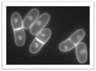
Figure 1. The fission yeast Schizosaccharomyces pombe. Fission yeast is an excellent model system. It is easy to grow in the laboratory, easy to transform, and it has a very small genome (12 Mb). It has ~5,000 protein-coding genes and ~1,500 non-coding RNAs. It is haploid. Fission yeast and the budding yeast Saccharomyces cerevisiae are not closely related fungi, so study of both has contributed greatly to our understanding of molecular biology, evolutionary biology, and quantitative genetics.
2.3 GWAS for yeast
GWAS is often used for human or crop traits, but we can apply this method to any sexually recombining eukaryotic species for which we have trait data and polymorphism data (e.g., SNPs).
The data we will use come from two papers: Nature Genetics and Nature Communications. These articles described the genetic diversity of 160 strains of this species by sequencing their genomes, and measured over 200 traits.
In this workshop we will examine GWAS results for four traits and consider what they could mean for the evolution of this species.
2.4 The traits
The traits we will look at today are:
Growth in 400 mM NaCl The growth rate of the strains in 400 mM salt. This could be important if strains grew in fruit near the sea or in salty substrates.
Growth at elevated temperature The growth rate of the strains at 40 °C. This is quite warm for this yeast, so it is a stressful condition.
Maximal cell density in rich medium This trait measures how well each strain grows when given plenty of sugar and other resources.
Glucose/fructose utilisation in wine How much of the glucose and fructose each strain used in grape must (used to make wine).
Traits and trade-offs
A high value in one of these traits could be adaptive in one environment but suboptimal in another. Also, optimising one trait may limit another trait. This could be because one mutation results in multiple changes, or the alleles that influence two traits are closely linked.
3 Exercises
3.1 Exploring the data
First, clear all the previous data you may have in R, set your working directory, and load the GWAS data.
To set a working directory you can either use a command (as below), or use the menus;
Session > Set Working Directory > Choose Directory.
After loading these data you will have four data frames called gluc, heat, rich, and salt. Each contains the GWAS results for one trait. Start by looking at salt.
Try these commands to see what they contain:
#examine what is in the salt data frame
head(salt)
nrow(salt)
summary(salt)
View(salt)
This table contains the output from a GWAS tool called LDAK. This is one of many software tools that run GWAS analyses. It describes the association of each SNP with the trait of salt tolerance.
Each row of the table contains information about one SNP. For our purposes, the important columns are:
Wald_P, the P-value, the probability that this SNP is associated with this traitChr, which chromosome the SNP is onBP, the position of the SNP in the chromosomeEffect_size, how strongly this variant affects the trait
The effect size of the variant estimates the proportion of trait variation that is explained by this SNP. From our understanding of the Neutral Theory of Molecular Evolution, we know that most variants are selectively neutral, i.e., they have little or no effect on fitness.
Given this, we might expect that most variants have small, or no, effects on traits.
3.2 Manhattan plot
A Manhattan plot is a standard way of viewing GWAS results. They are named Manhattan plots because they resemble the skyline of a high-rise city, such as Manhattan (New York).
Manhattan plots show the position of the SNP on the x-axis, and the P-value of the association on the y-axis. P-values are plotted as −log10(P), so that very small P-values end up at the top of the plot and stand out.
The code below will make a Manhattan plot for the salt trait.
#set plotting parameters
layout(matrix(c(1:3), 1, 3, byrow = TRUE),widths = c(5579133,4539804,2452883))
par(bty="l",cex=0.8,mar=c(2,2,2,0)+2)

#loop through chromosomes 1,2,3, plotting each one in turn
for (j in 1:3){
      #make a subset of SNPs from this chromosome
      temp = subset(salt, Chr == j)
      #plot these
      plot(temp$BP, -log10(temp$Wald_P),
           main = paste("Chr",j),ylim=c(1,10),
           xlab="position",ylab="-log10(P)"
      )
      #draw a threshold line
      #SNPs above this line are statistically associated with the trait
      abline(h=-log10(1e-5),col=2,lty=2)
}
Discussion points: Manhattan plot
- Where are the strongest association signals located (do peaks cluster on particular chromosomes)?
Answer: Association signals located on all chromosomes.
- Why are most points close to the bottom of the plot? What does this tell you about polygenic traits?
Answer: Most points close to the bottom of the plot because most SNPs are not strongly associated with the trait. This, and the fact that we see signals located on all chromosomes tells us that there can be many genetic variants that affect traits, but most affect traits very weakly, if at all.
- How does the −log10(P) scale aid interpretation compared to plotting raw P-values?
Answer: This method highlights the very small P-values (which will be high up on the y axis), which in this case is what we want to see.
- What biological processes could lead to a few tall peaks versus many low signals (e.g., selection, drift, mutation rate, linkage)?
Answer: Selection might lead to this effect. If alleles were present that had strong effects on traits, but they had not yet swept to fixation.
You will usually see a small number of very low P-values; with large −log10 values they sit at the top of the y-axis. For these, there is strong support that they affect the trait.
You will also see many SNPs with P-values around 0.1 or greater. These are at the bottom of the y-axis. There is weak support that they affect the trait. These may have tiny effect sizes, or none at all.
−log10 scale plotting
Note that we use plot(temp$BP, -log10(temp$Wald_P)) to plot the Wald_P P-values on a negative log scale. This means that very significant P-values (e.g., P = 1 × 10^−9.5) will show as high points on the plot (e.g., at position 9.5 on the vertical y-axis in this case).
All the non-significant SNPs (e.g., P = 0.1, which is 1 × 10^−1) will be at the bottom of the y-axis. If most variants have small or no effects on traits, there will be many of these.
This illustrates polygenic architecture: many variants with small effects and a few with larger effects.
3.3 SNP effect sizes
The strength of the association between genotype and phenotype relates to the effect size (how strongly the variant affects the trait). Some alleles affect the trait strongly; most do not. Now make a histogram of all the effect sizes.
hist(salt$Effect_size,br=30)
Discussion points: effect sizes
- What does the histogram shape tell you about the distribution of SNP effect sizes?
Answer: The vast majority of SNPs that we find in genetic diversity in this set have small effects on traits.
- How does this pattern relate to the Neutral Theory (many neutral or near-neutral variants)?
Answer: This is consistent with the Neutral Theory, because if most SNPs have no effect on traits they are unlikely to affect fitness (so will be fitness-neutral).
- Where would you expect to see evidence of purifying selection or positive selection in such a distribution?
Answer: For a trait that has some relevance to fitness, purifying selection should reduce the effect sizes of SNPs.
3.4 How does this influence evolution?
Effect size here is the proportion of phenotypic variance explained by that SNP. Most effect sizes are very small—often < 0.05—meaning each explains far less than 5% of the trait variance.
Consider how such tiny-effect alleles influence evolutionary change.
A selective sweep is a process where a beneficial mutation becomes fixed in a population rapidly, removing the genetic variation around the selected allele.
Discussion points: selective sweeps and polygenicity
- If a trait is influenced by a few large-effect mutations, how likely is a classic selective sweep and why?
Answer: In this case a classic selective sweep is more likely, because selection will be acting strongly on those few SNPs, so their allele frequencies would be expected to change rapidly, thereby removing the genetic variation around them.
- If a trait is influenced by many tiny-effect mutations, what evolutionary pattern replaces a sweep? (Think subtle allele frequency shifts.)
Answer: In an extreme example (where much of the genome is subject to selection), we would not expect to observe the genomic signatures of selective sweeps. So, in this case a classic selective sweep seems less likely.
- How can tight linkage to a deleterious allele modify or slow a sweep?
Answer: If an advantageous SNP is very close to a deleterious SNP, and on the same haplotype, it might not change frequency at all.
- What genomic signatures (e.g., reduced diversity, extended haplotype homozygosity) would differ between oligogenic and highly polygenic adaptation?
Answer: Reduced diversity would be less obvious in highly polygenic adaptation, as it is difficult to distinguish from stochastic variation in diversity.
3.5 Another trait: glucose & fructose use
In a vineyard environment, it is advantageous to metabolise glucose and fructose in rotting fruit. Glucose/fructose use is in the gluc data frame.
Again, we will look at the P-values (Wald_P) and how much each SNP is predicted to affect the trait (Effect_size).
#set plotting parameters
layout(matrix(c(1:3), 1, 3, byrow = TRUE),widths = c(5579133,4539804,2452883))
par(bty="l",cex=0.8,mar=c(2,2,2,0)+2)

#loop through chromosomes 1,2,3, plotting each one in turn
for (j in 1:3){
      temp = subset(gluc, Chr == j)
      plot(temp$BP, -log10(temp$Wald_P),
           main = paste("Chr", j, "Gluc"),ylim=c(1,10),
           xlab="position",ylab="-log10(P)"
      )
      abline(h=-log10(1e-5),col=2,lty=2)
}
Discussion points: second trait comparison
- Do the strongest glucose/fructose association peaks overlap with salt peaks? What could shared loci imply (pleiotropy vs linkage)?
Answer: While the strongest signals do not generally overlap, there are some cases where they do. This could imply that the same genetic variants influence both traits (pleiotropy), or that they are linked (i.e., on the same haplotype).
- Are there trait-specific peaks? What might that say about specialised metabolic pathways?
Answer: Yes, there are trait-specific peaks. This suggests that some genetic variants influence only one trait, perhaps because they are involved in specialised metabolic pathways.
- How could environmental context (salinity vs sugar availability) shift which alleles are favoured?
Answer: If the organism (yeast, in this case) moves from one environment to another, or if the environment changes (e.g., the soil becomes more saline or more sugary), different alleles may be favoured by selection, depending on which traits are more important for survival and reproduction in that context.
Again, you will see a small number of very low P-values at the top of the y-axis (strong support) and many higher P-values at the bottom (weak or no support; tiny or no effect sizes).
Now, make a histogram of the effect sizes:
hist(gluc$Effect_size)3.6 Looking at two traits
Species cannot adapt to a single condition (e.g., heat or salt) in isolation because environments are complex and variable. As a thought experiment, we will consider this using the fission yeast data.
We will compare two Manhattan plots by overlaying them: salt (black) and glucose/fructose metabolism (red). The output PDF will appear in your working directory.
#open the pdf writer
pdf("GWAS-plot3.pdf",width=60)
#set up the plot layout
layout(matrix(c(1:3), 1, 3, byrow = TRUE),widths = c(5579133,4539804,2452883))
par(bty="l",cex=0.8,mar=c(2,2,2,0)+2)
#loop through chromosomes
for (j in 1:3){
      #plot the salt GWAS points (black dots)
      temp = subset(salt, Chr == j)
      plot(temp$BP, -log10(temp$Wald_P),main = "",ylim=c(1,10),xlab="position",ylab="-log10(P)")

      #add the glucose/fructose GWAS points (red crosses)
      temp2 = subset(gluc, Chr == j)
      points(temp2$BP, -log10(temp2$Wald_P),main = "gluc",ylim=c(1,10),xlab="position",ylab="-log10(P)",col=2,pch=3)

      #add the significance threshold
      abline(h=-log10(1e-5),col=2,lty=2)
}
#close the pdf writer
dev.off()
Now find the pdf called GWAS-plot3.pdf and take a look.
3.6.1 Might mutations for two traits conflict?
Look at the significant peak on chromosome 3 (~1,500,000 bp). This likely has a relatively large effect size. There is also an important variant for glucose/fructose use nearby on chromosome 3.
Consider what might happen if alleles are linked and the environment is complex—salty yet fructose-rich (e.g., a coastal vineyard).
What might happen if helpful alleles for both traits are on the same haplotype?
Haplotypes
Physically, a haplotype is a stretch of DNA from one chromosome. In diploids, each individual carries two homologous chromosomes. In haploid S. pombe, different haplotypes are simply different chromosome versions present across the population. Through meiotic recombination haplotypes mix, but SNPs very close together rarely separate, so they tend to travel together.
3.6.2 Haplotype problems
Consider these situations:
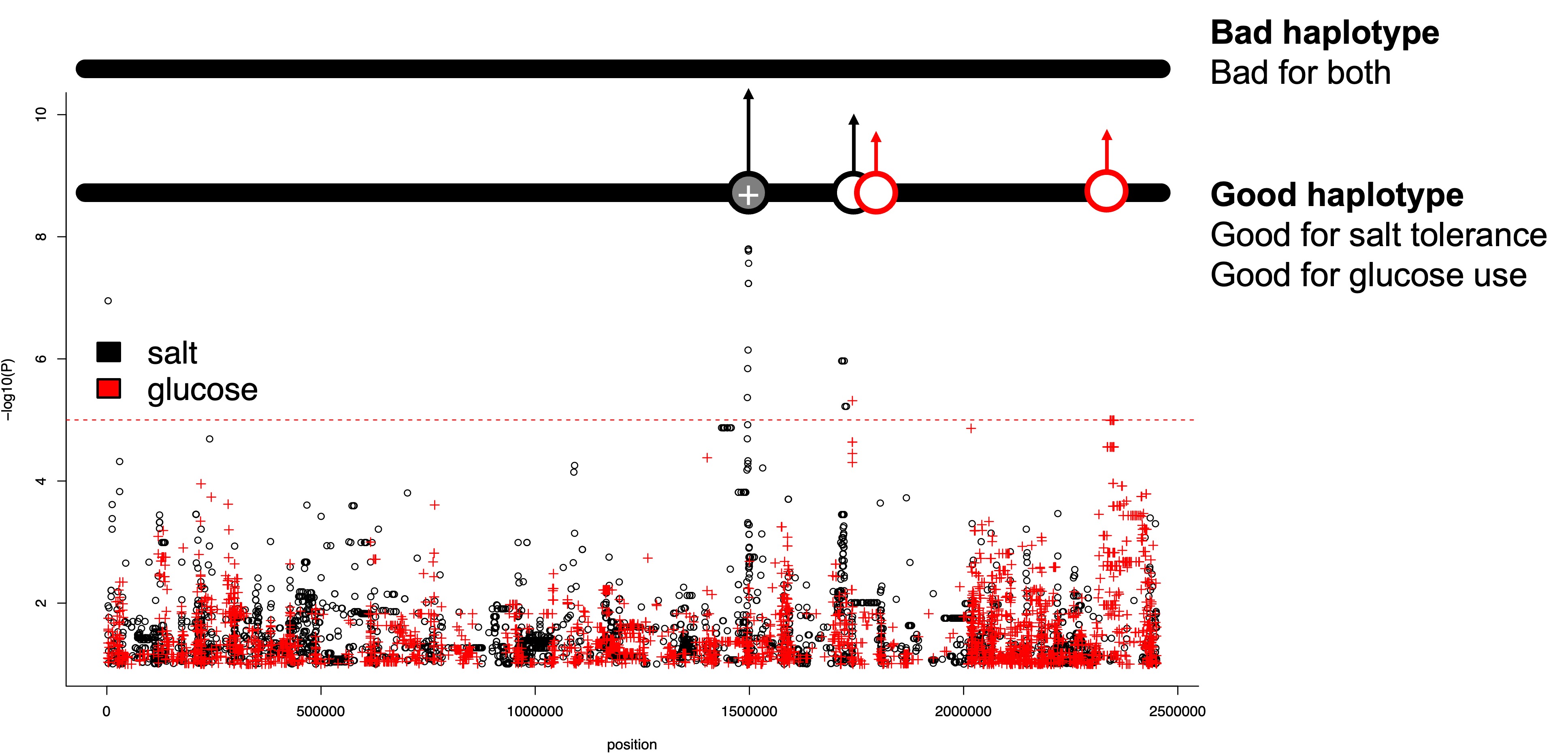
- What might happen if helpful alleles are on the same haplotype?
- What might happen if helpful alleles are on different (opposing) haplotypes?
The figures below will help to explain.
Discussion points: haplotypes and linkage
- How does tight linkage between beneficial alleles influence the speed of joint adaptation?
Answer: Tight linkage between beneficial alleles can facilitate rapid joint adaptation, as selection can act on the combined effect of the linked alleles.
- What evolutionary constraint arises when beneficial alleles are on different haplotypes in low recombination regions?
Answer: When beneficial alleles are on different haplotypes in low recombination regions, selection on one allele can interfere with the selection on the other, slowing down the overall adaptation process.
- How can recombination rate modulate the resolution of this “conflict” between opposing haplotypes?
Answer: Higher recombination rates can help to separate linked alleles, allowing beneficial alleles on different haplotypes to be combined into a single haplotype, thereby resolving the conflict.
- Which scenario (single vs opposing haplotypes) better facilitates rapid multi-trait optimisation?
Answer: The single haplotype scenario better facilitates rapid multi-trait optimisation, as it allows for the simultaneous selection of beneficial alleles for both traits without interference.
Figure 2. Beneficial alleles on one haplotype. Would there be any conflict here?
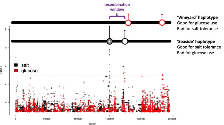 Figure 3. Beneficial alleles on two different haplotypes. What might happen here? What is the potential problem?
4 Summary: what we have learned
This workshop used data from fission yeast, but the principles apply broadly to quantitative traits. Key points:
- Most SNPs do not strongly associate with traits.
- Most SNPs have very small effects on traits, but some do have detectable effects.
- SNPs do not affect all traits at once. Some SNPs affect one trait; some affect another.
- Genetic variants, like SNPs, travel through time and space in haplotypes.
5 After the workshop: exam-style questions
Exam questions often ask you to apply workshop principles to other species or scenarios. Reflecting on these helps deepen understanding.
Principles of quantitative genetics
- Most SNPs have no effect, or very small effects, on traits.
- SNPs that do affect traits are generally responsible for less than 5% of the trait variation.
- Effect sizes are also small for other genetic variants, such as transposon insertions, duplications/deletions and so on.
- Genetic variants can affect one trait, or several.
- In the short term, selection occurs on haplotypes, but over time recombination will separate linked variants.
5.1 Question 1 (10 points)
This question checks your understanding of quantitative traits and why most variants have small effects.
- Define the difference between a simple (single-gene) trait and a quantitative trait. Give one example of each from this workshop. (2 points)
Answer: A simple (single-gene) trait is controlled by one gene, where a mutation in that gene can lead to a distinct phenotype. An example from this workshop could be a hypothetical mutation in a gene that confers resistance to a specific toxin. A quantitative trait is influenced by multiple genes, each contributing a small effect to the overall phenotype. An example from this workshop is salt tolerance, which is affected by many SNPs with small effect sizes.
- The histogram of SNP effect sizes for the salt trait is heavily skewed towards zero. Describe what this pattern tells us about the distribution of SNP effects in the population. (3 points)
Answer: The histogram indicates that the majority of SNPs have very small or negligible effects on the salt tolerance trait. This suggests that most genetic variation in the population does not significantly influence this trait, while only a few SNPs have larger effects. This pattern is consistent with the idea that quantitative traits are polygenic, with many loci contributing small effects rather than a few loci having large effects.
- Using the Neutral Theory of Molecular Evolution, explain why most SNPs are expected to have little or no effect on fitness. (3 points)
Answer: The Neutral Theory of Molecular Evolution posits that most genetic variation is neutral with respect to fitness, meaning that it does not affect an organism’s ability to survive and reproduce. There are several reasons for this;
- From molecular biology, we know that synonymous mutations (that do not change the protein sequence) are unlikely to affect fitness. Even nonsynonymous mutations in coding regions (that do change the protein sequence) generally have small effects on fitness, because we are altering just one amino acid within the 5,000 protein-coding genes of fission yeast.
- From population genetics, we know that deleterious mutations are removed by purifying selection, and beneficial mutations are rare and often fixed rapidly by positive selection.
- So, most SNPs that persist in the population are either neutral or nearly neutral, leading to the expectation that most SNPs will have little or no effect on fitness.
- Suggest one practical way to increase the power of a GWAS to detect very small-effect variants and explain why it helps. (2 points)
Answer: Increase the sample size of the study population. A larger sample size increases the statistical power to detect associations between SNPs and traits.
5.2 Question 2 (10 points)
You notice that the Manhattan plots for salt tolerance and glucose/fructose utilisation share a peak on chromosome 3, but also have trait-specific peaks.
- Describe what an overlapping peak for both traits suggests about the underlying genetics of those traits. (3 points)
Answer: An overlapping peak for both traits suggests that there may be a shared genetic basis influencing both salt tolerance and glucose/fructose utilisation. This could indicate pleiotropy, where a single genetic variant affects multiple traits, or it could suggest that the two traits are influenced by closely linked genetic variants located near each other on the chromosome.
- State one additional analysis you could carry out to test whether the same causal variant influences both traits. (2 points)
Answer: We could use CRISPR-Cas9 gene editing to create targeted mutations in the candidate gene(s) located within the overlapping peak region. By observing the effects of these mutations on both salt tolerance and glucose/fructose utilisation, we can determine if the same causal variant influences both traits.
- Explain how recombination could help resolve a situation where beneficial alleles for two traits are on different haplotypes. (3 points)
Answer: Recombination during meiosis can shuffle genetic variants between homologous chromosomes, allowing beneficial alleles for different traits that are initially on separate haplotypes to be brought together onto the same haplotype. This process can create new combinations of alleles that confer advantages for both traits simultaneously, thereby resolving the conflict between opposing haplotypes and facilitating multi-trait optimisation.
- Identify one environmental measurement you would collect alongside the genomic data to interpret potential trade-offs between the two traits, and justify your choice. (2 points)
Answer: All of the experiments in this workshop relate to salt tolerance and sugar metabolism in the laboratory. Therefore, we would collect data on environmental salinity levels in the natural habitats where S. pombe is found, and measure environmental salinity. Justification: The workshop emphasizes that species face complex, multivariable environments—illustrated by the example of a “coastal vineyard” that is both salty and fructose-rich. By measuring natural salinity levels in the fruiting environments we could determine how the laboratory experiments might relate to the natural environment.